GWAS

Introduction

Genome-wide Association Study (GWAS) is a classic methodology for identifying SNPs associated with common diseases. By scanning the entire genome without prior hypotheses, it utilizes linear models to identify SNPs with significant statistical associations to specific diseases. However, because allele frequencies vary across populations and current GWAS data are predominantly derived from European ancestry, the predictive performance across different ethnic groups remains limited. Furthermore, due to Linkage Disequilibrium (LD), the significant loci identified by GWAS are often merely “tagging SNPs” rather than the actual causal variants responsible for the disease.

During the Quality Control (QC) process, SNPs with a low Minor Allele Frequency (MAF) are typically excluded. Rare variants have extremely low frequencies; for instance, a MAF of 0.01 implies that, on average, only one individual out of 100 carries that specific SNP. When the sample size of a study is insufficient, the influence of these few rare-variant carriers often fails to reach the stringent p-value threshold required for genome-wide significance.

Material and Method

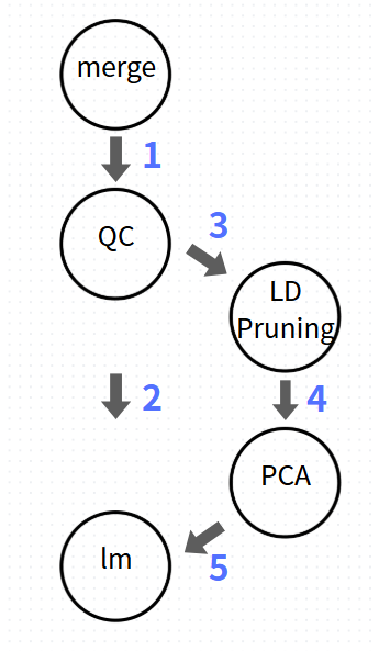
The GWAS workflow begins with stringent QC based on MAF and Hardy-Weinberg Equilibrium (HWE). Following QC, the filtered SNPs are used for the primary association analysis. For population structure correction, a subset of SNPs is subjected to LD pruning to perform Principal Component Analysis (PCA). The final Linear Regression Model incorporates the post-QC SNPs as the independent variable, with Principal Components (PCs) and gender included as covariates to account for population stratification and confounding factors.

Data

We utilized data from the 1,000 Genomes Project to perform a GWAS for height. The study encompassed chromosomes 1 through 22, analyzing a total of 36,820,992 variants across 1,092 individuals.

Genotype QC

Excluding the SNP or individual with missing rate $> 0.1$ : 36820992 variants and 1092 people pass filter
Excluding the SNP with MAF $\leq 0.05$ : 6797981 variants and 1092 people pass filter
Excluding the SNP with HWE $< 0.0001$ i.e. pvalue $< 0.0001$ : 4941621 variants and 1092 people pass filter
Excluding the SNP with $r^2 < 0.2$ in 500 window bp to PCA : 299901 variants and 1092 people pass filter

Linear model

After applying filters for missingness rate, MAF, and HWE, the dataset retained 4,941,621 variants and 1,092 individuals. This high-quality dataset served as the foundation for constructing the linear model

$$ \begin{align*} Y_i &= X_j + Gender + {PC}_1 + {PC}_3 + {PC}_3,\\ i &=1, \cdots , 1092; \quad j=1, \cdots , 299901 \end{align*} $$

where $Y_i$ is i-th sample, $X_j$ is j-th SNP.

Result

SNP Finding

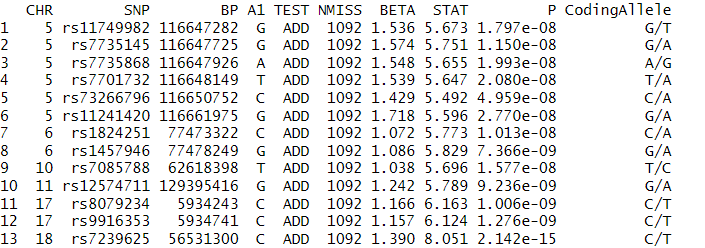
We identified several SNPs significantly associated with height, using the standard threshold of p-value $< 5 \cdot 10^{-8}$. These lead SNPs and their corresponding statistics are summarized in the table below.

LD

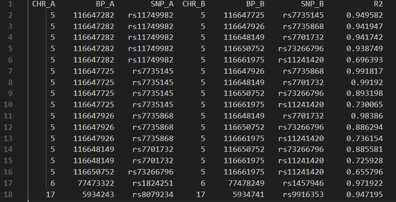
To determine if multiple significant SNPs represent the same underlying genetic signal, we evaluated the LD between them. Our analysis indicates that five significant SNPs on Chromosome 5 are in high LD with one another, suggesting they likely tag the same causal locus. Similarly, high LD was observed between two SNPs on Chromosome 6, as well as two SNPs on Chromosome 17.

Manhattan Plot

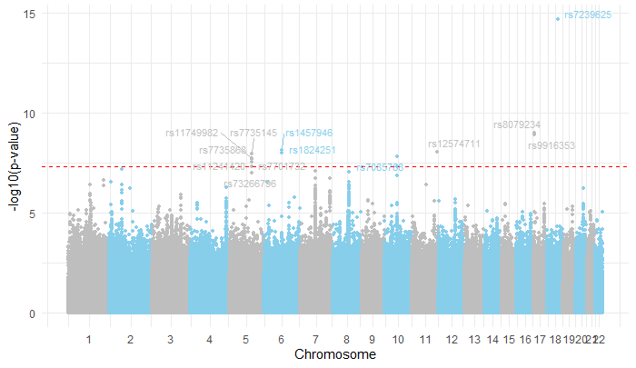
The Manhattan plot visualizes the association results across the genome, with the red dashed line indicating the significance threshold ($-\log_{10}(5 \cdot 10^{-8})$). The plot highlights prominent peaks of significant SNPs, most notably on Chromosome 5, which demonstrates the strongest association with the trait.

Code

1
2
library(data.table)
library(dplyr)

merge data

 1
 2
 3
 4
 5
 6
 7
 8
 9
10
11
12
13
14
15
16
17
18
19
20
21
22
23
24
setwd("D:/GWAS_CLASS/midterm")

for (i in 1:22) {
  ## vcf to bed
  paste0("plink --vcf ALL.chr" ,i ,".phase1_release_v3.20101123.snps_indels_svs.genotypes.vcf.gz --make-bed --out chr", i ) %>%
    system()

  ## 把snp id是.的轉換成新的名稱
  paste0("plink --bfile chr", i, " --snps-only just-acgt --set-missing-var-ids @:#[b37] --make-bed --out chr", i, "_TransformMissing") %>%
    system()
}


list <- list()
for (i in 2:22) {
  ## merge files
list<- list %>%
  rbind(paste("chr", i, "_TransformMissing",c(".bed",".bim",".fam"),sep=""))
}
## 造merge_files.txt，放你要合併的檔案名稱
write.table((list),file="merge_files.txt",row.names=F,col.names=F,quote=F)

## 把chr22_1_1的bed,bim,fam 跟merge_files.txt 裡的合併
system("plink --bfile chr1_TransformMissing --merge-list merge_files.txt --make-bed --out process//merge")

QC and LD and PCA

 1
 2
 3
 4
 5
 6
 7
 8
 9
10
11
12
13
14
15
16
17
18
19
20
21
22
23
24
25
26
27
28
29
30
31
32
33
setwd("D:/GWAS_CLASS/midterm")

## 產生兩個檔案，分別紀錄人跟snp missing 的檔案
system("plink --bfile process/merge --missing" )

# 把人missing rate 超過0.1 的人 丟掉
system("plink --bfile process//merge --mind 0.1 --geno 0.1 --maf 0.05 --hwe 0.0001 --make-bed --out process//merge_QC" )

# 轉成ped, map
system("plink --bfile process//merge_QC --recode --out process//merge_QCPed" )

#ld pruning(只輸出prune.in, prune.out)
system("plink --file process//merge_QCPed --indep-pairwise 500 50 0.2 --out process//merge_QCld")

# choose SNP in prune.in, output .ped and .map
system("plink --file process//merge_QCPed --extract process//merge_QCld.prune.in --recode --out process//merge_prune")

#pca
system("plink --file process//merge_prune --pca --out process//merge_pca")


e.vec <- fread("process//merge_pca.eigenvec")

g <- fread("process//pheno.txt")
covar <- data.frame(FID = e.vec$V1,
                    IID = e.vec$V2,
                    gender = g$Gender,
                    PC1 = e.vec$V3,
                    PC2 = e.vec$V4,
                    PC3 = e.vec$V5)


write.table(covar,file="D://GWAS_CLASS//20101123//process//covar.txt",row.names=F,quote=F)

1
2
3
4
5
## association
### 千萬要注意!!!pheno.txt 檔案顯示成文字檔，每個row文字要用tab區隔，也就是說用記事本打開，看起來不會是對齊的
system("plink --bfile process//merge_QC --pheno process//pheno.txt --pheno-name Height --make-bed --out process//merge_f" )
##
system("plink --bfile process//merge_f --covar process//covar.txt --covar-name gender PC1 PC2 PC3 --allow-no-sex --linear --out process//linear_model" )

choose sig SNP

 1
 2
 3
 4
 5
 6
 7
 8
 9
10
11
12
13
14
15
16
17
18
19
20
21
22
23
24
## plot
r <- read.table(file="process//linear_model.assoc.linear", header = T)
head(r)
loc <- fread("process//merge_f.bim", header = F)

# 合併v5,v6
loc <- loc %>%
  mutate(CodingAllele = paste(V5, V6, sep = "/"))

names(loc)[1:4] <- c("CHR","SNP","v3","BP")


## 有4941621 個snp，只取線性模型裡的ADD term
r_snp <- r[1+5*(0:4941620),]
dim(r_snp)
head(r_snp)

dim(r)
dim(loc)


snp_sig <- r_snp[which(r_snp$P<5*10^(-8)), ]
snp_sig <- snp_sig %>%
  left_join(loc %>% select(SNP, CodingAllele), by = "SNP")

sig SNP is LD high?

 1
 2
 3
 4
 5
 6
 7
 8
 9
10
11
12
prune_out <- fread("process\\merge_QCld.prune.out")
snp_sig_ld <- intersect(snp_sig$SNP, prune_out)
snp_sig_ld

sig <- data.frame(sig_snp = snp_sig$SNP)
write.table(sig, file="process//significant_snp.txt", row.names=F, col.names=F, quote=F)

# select significant_snp.txt snp in merge_QCPed
system("plink --file process//merge_QCPed --extract process//significant_snp.txt --recode --out process//merge_sig")

# get all pairs ld
system("plink --file process//merge_sig --r2 --ld-window-r2 0 --out process//sig_snp_LD")

plot

 1
 2
 3
 4
 5
 6
 7
 8
 9
10
11
12
13
14
15
16
17
18
19
20
21
22
23
24
25
26
27
28
29
30
library(ggplot2)
library(dplyr)
library(ggrepel)  # 為避免標籤重疊

# 計算 -log10(p-value)
r_snp$logP <- -log10(r_snp$P)

# 建立 i 軸 (x 軸索引)
r_snp <- r_snp %>% arrange(CHR, BP) %>%
  mutate(i = 1:n())

# 取得每個染色體中間位置，當作 x 軸刻度的位置
chr_labels <- r_snp %>%
  group_by(CHR) %>%
  summarize(center = median(i))

# 篩選出顯著 SNP（p < 5e-8）
sig_snps <- r_snp %>% filter(P < 5e-8)

# 畫圖
ggplot(r_snp, aes(x = i, y = logP, color = as.factor(CHR %% 2))) +
  geom_point(size = 1) +
  scale_color_manual(values = c("skyblue", "grey")) +
  geom_hline(yintercept = -log10(5e-8), color = "red", linetype = "dashed") +
  scale_x_continuous(breaks = chr_labels$center, labels = chr_labels$CHR) +
  labs(x = "Chromosome", y = "-log10(p-value)", title = "Manhattan Plot") +
  theme_minimal() +
  theme(legend.position = "none") +
  # 加上 SNP 標籤
  geom_text_repel(data = sig_snps, aes(label = SNP), size = 3, max.overlaps = 20)

Next Steps

Following the GWAS, several post-GWAS analyses can be conducted, including fine-mapping, functional annotation, and the calculation of polygenic risk scores (PRS). Furthermore, the GWAS catalog provides a vast repository of existing GWAS summary statistics. We can leverage this data to validate the significant SNPs identified in our study.

Reference

1000G
Prof. lhchien Course