Censored and Truncated
Censored
Event occurs before the observing starting time, event time left to starting time. we called it left censored. For example, event is getting disease. A sample have already got it before we observe it. It is left censored data.
Event occurs after the observing ending time, event time right to ending time. we called it right censored. For example, a sample doesn’t get it until we stop observing. It is right censored data.
When data both left and right censored, we call double censored.
Truncated
The idea is quit similar to censor. Censored data is observed the kind of data but it doesn’t complete. Truncated data is that we will not use the incomplete data as a simple.
We only observe the data with event occuring after starting time, so we truncate those event left to starting time. Those data we called it left truncated.
We only observe the data with event occuring before ending time, so we truncate those event right to ending time. Those data we called it right truncated.
When data both left and right truncated, we call double truncated.
Basic Code
survfit(Surv(time1,time2,delta)~type, data = tongue):
We classify tongue by different type (No type we use 1); censored time from time1 to time2. delta means event, normally 0=alive, 1=dead.
| |
| |
time ($t_i$):發生 event 的時間點,也就是存活函數的跳點
n.risk ($Y_i$):在 $t_i^{-}$ 時還活著的人,包含在 $t_i$ 發生 event 的人
n.event ($d_i$):在 $t_i$ 發生 event 的人數
survival ($\hat{S(t_i)}$):K.M. estimator
std.err:$\hat{S(t_i)}$的standard error ,使用 Greenwood’s formula 算出
cumhaz:N.A. estimator,碰到censored的 $t_i$ 時,值不變
Left-Truncated
資料從左邊切斷,像是從資料的變數 ageentry 從 $(80 * 12)$ 開始看
| |
Censoring
Right-censored
假設總有一天會發生事件,而且發生在觀察時間的右邊
Left-censored
事件發生在觀察時間的左邊,像是毒癮者,接受治療前已經開始使用毒品
Interval-censored
事件發生在兩個觀察時間之間,像是每隔10小時才觀察一次,只知道事件發生的時間區間。
Estimator
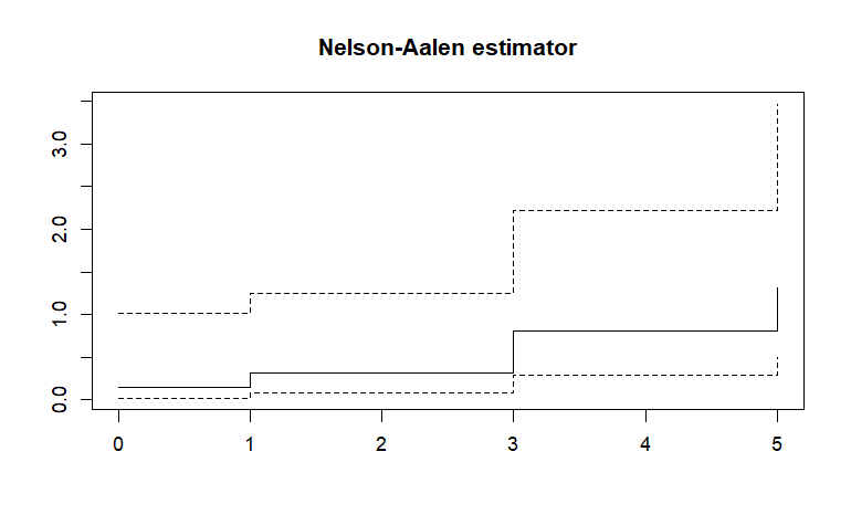
Nelson-Aalen estimator
$$\begin{align*} \overset{\sim}{H(t)} = \left \lbrace \begin{array}{lll} \ \ 0 & \text{if} & t \leq t_1 \\\\\\ \displaystyle \sum_{t_i \leq t} \frac{d_i}{Y_i} & \text{if} & t \geq t_1 \end{array} \right. \\\\\\ \end{align*}$$ | |
在有事件發生時,cummulative hazard 馬上往上跳;碰到censored的 $t_i$ 時,值不變。所以是個右連續的階梯函數。(每一段的實心點在左端點)
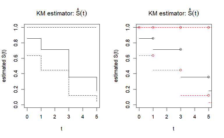
KM estimator
$$\begin{align*} \hat{S(t)} = \left \lbrace \begin{array}{lll} \ \ 1 & \text{if} & t < t_1 \\\ \displaystyle \prod_{t_i \leq t} (1- \frac{d_i}{Y_i}) & \text{if} & t \geq t_1 \end{array} \right. \\\ \end{align*}$$ | |
Proportional Hazard Model (Cox)
$Z_1:I(女)$
$Z_2:I(黑人)$
$Z_3:I(Z_1 \times Z_2)$
4 groups: black female, black male, white female, white male
Baseline
Baseline is $Z_1,\ Z_2,\ Z_3$ are $0$. It means white male.
Hazard ratio
$$\begin{align*} \frac{h(t\ |\ \text{black male})}{h(t \ |\ \text{white male})} &= \frac{h(t|(Z_1,Z_2,Z_3)=(0,1,0))}{h(t|(Z_1,Z_2,Z_3)=(0,0,0))} \exp{(\beta_2)} \\\ & = \exp{(-0.08878)} \\\ & =0.92 \\\ \end{align*}$$$$\begin{align*} \frac{h(t\ |\ \text{black male})}{h(t \ |\ \text{white female})} &= \frac{h(t|(Z_1,Z_2,Z_3)=(0,1,0))}{h(t|(Z_1,Z_2,Z_3)=(1,0,0))} \exp{(\beta_2 - \beta_1)} \\\ & = \exp{(-0.08878+0.24848)} \\\ & =1.17 \\\ \end{align*}$$ | |
Outcome
| |
Conditional Survival function
$$\begin{align*} \hat{S(t)}= \prod_{a \leq t_i \leq t} 1- \frac{d_i}{Y_i} ,\ t \geq a \\\\\\ \end{align*}$$ | |
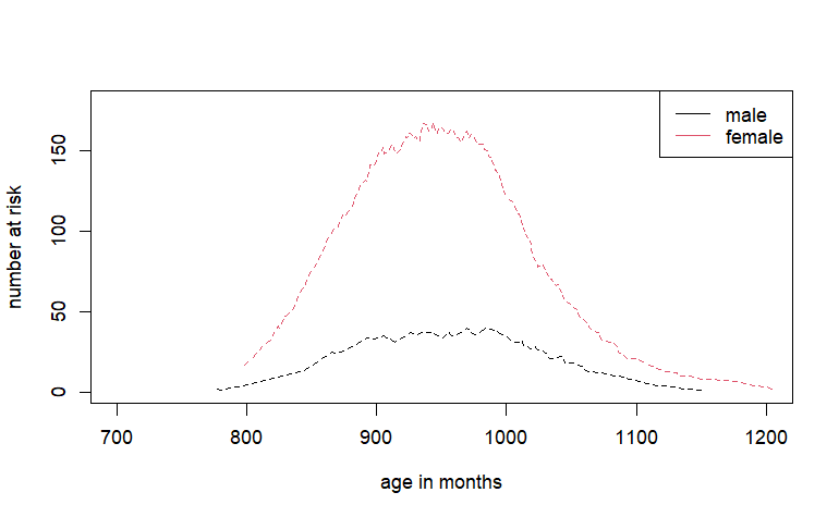
Risk plot
| |
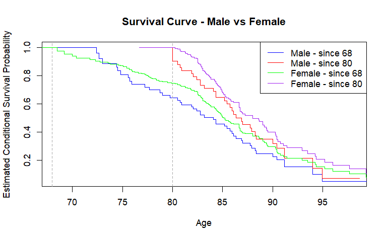
Survival Function for Left-truncated data
分別觀察68與80歲以上的生存曲線,left-truncated at 68 and 80
| |