$$Y_i = \beta_0+ \beta_1 x_{i,1} + \cdots + \beta_{p-1} x_{i,p-1} + \varepsilon_i, \quad \varepsilon_i \sim N (0, \sigma_i^2) $$$$\frac{Y_i}{\sigma_i} = \frac{1}{\sigma_i} (\beta_0+ \beta_1 x_{i,1} + \cdots + \beta_{p-1} x_{i,p-1} + \varepsilon_i), \quad \frac{\varepsilon_i}{\sigma_i} \sim N (0, 1) $$$$\begin{align*}
& Y
= \begin{pmatrix}
Y_1 \\\\\\
Y_2 \\\\\\
\vdots \\\\\\
Y_n
\end{pmatrix},
\ X
= \begin{pmatrix}
1 & x_{11} & \cdots & x_{1, p - 1} \\\\\\
1 & x_{21} & \cdots & x_{2, p - 1} \\\\\\
\vdots & \vdots & \ddots & \vdots \\\\\\
1 & x_{n1} & \cdots & x_{n, p - 1} \\\\\\
\end{pmatrix},
\ \varepsilon
= \begin{pmatrix}
\varepsilon_1 \\\\\\
\varepsilon_2 \\\\\\
\vdots \\\\\\
\varepsilon_n
\end{pmatrix},
\ \beta
= \begin{pmatrix}
\beta_0 \\\\\\
\beta_1 \\\\\\
\vdots \\\\\\
\beta_{p-1}
\end{pmatrix} \\\\\\
& W
= \begin{pmatrix}
1 / \sigma_1^2 & 0 & \cdots & 0 \\\\\\
0 & 1 / \sigma_2^2 & \cdots & 0 \\\\\\
\vdots & \vdots & \ddots & \vdots \\\\\\
0 & 0 & \cdots & 1 / \sigma_n^2 \\\\\\
\end{pmatrix},
\ Y_W = W^{\frac{1}{2}} Y,\ X_W = W^{\frac{1}{2}} X
\end{align*}$$$$\begin{align*}
\tilde{\beta}
& = \arg min \sum_{i = 1}^{n} \frac{(Y_i - \beta_0 - \beta_1 x_{i,1} - \cdots - \beta_{p - 1} x_{i, p - 1})^2}{\sigma_i^2} \\\\\\
& = \arg min (Y-X \beta)^{'}
\begin{pmatrix}
1 / \sigma_1^2 & 0 & \cdots & 0 \\\\\\
0 & 1 / \sigma_2^2 & \cdots & 0 \\\\\\
\vdots & \vdots & \ddots & \vdots \\\\\\
0 & 0 & \cdots & 1 / \sigma_n^2 \\\\\\
\end{pmatrix}
(Y-X \beta) \\\\\\
& = \arg min (Y-X \beta)^{'} W (Y-X \beta) \\\\\\
& = \arg min (W^{\frac{1}{2}} Y - W^{\frac{1}{2}} X \beta )^{'} (W^{\frac{1}{2}} Y - W^{\frac{1}{2}} X \beta ) \\\\\\
& = \arg min (Y_W - X_W \beta)^{'} (Y_W - X_W \beta)
\\\\\\
& = \arg min \left[(Y_W)^{'} Y_W - 2\beta^{'} (X_W)^{'} Y_W + \beta^{'} (X_W)^{'} X_W \beta \right] \\\\\\
& = \arg min Q(\beta)
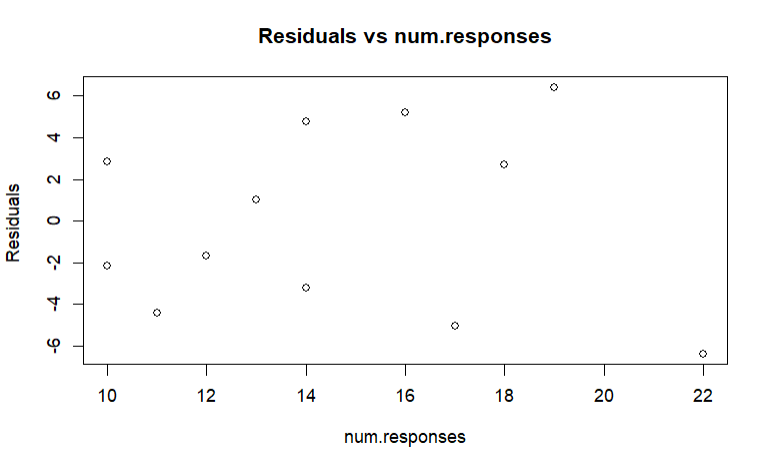
\end{align*}$$$$\left[- 2(X_W)^{'} Y_W + 2 (X_W)^{'} X_W \tilde{\beta} \right] = 0$$$$\tilde{\beta} = ((X_W)^{'} X_W)^{-1} (X_W)^{'} Y_W = (X^{'} W X)^{-1} X^{'} W Y$$A plot of $e_i$ against $X_i$ or $e_i$ against $\hat{Y_i}$ exhibits a megaphone shape. Regress $|e_i|$ against $X_i$ or regress $|e_i|$ against $\hat{Y_i}$. And we use the fitted value of the regression $\hat{|e_i|}$ to estimate $\sigma_i$ .
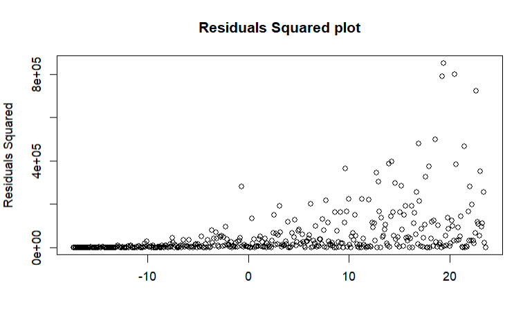
A plot of ${e_i}^2$ against $X_i$ or ${e_i}^2$ against $\hat{Y_i}$ exhibits an upward tendency. Regress ${e_i}^2$ against $X_i$ or regress ${e_i}^2$ against $\hat{Y_i}$. And we use fitted value of the regression $\hat{{e_i}^2}$ to estimate ${\sigma_i}^2$.
Example
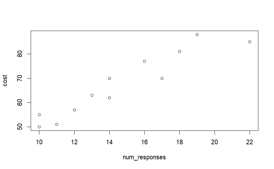
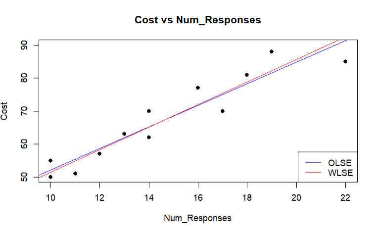
The response $Y$ is the cost of the computer time and the predictor $X$ is the total number of responses in completing a lesson. The data downloaded from(https://online.stat.psu.edu/stat501/lesson/13/13.1/13.1.1).
Plot $e$ v.s. $X$, it shows a megaphone shape.
The variance of ordinary model is not constant. We regress $|e|$ v.s. $X$, then we use $\hat{|e_i|}$ to estimate $\sigma_i$. Therefore, $w_i=\frac{1}{{|e_i|}^2}$.
Compare the OLSE and WLSE. It’s just a little bit different.
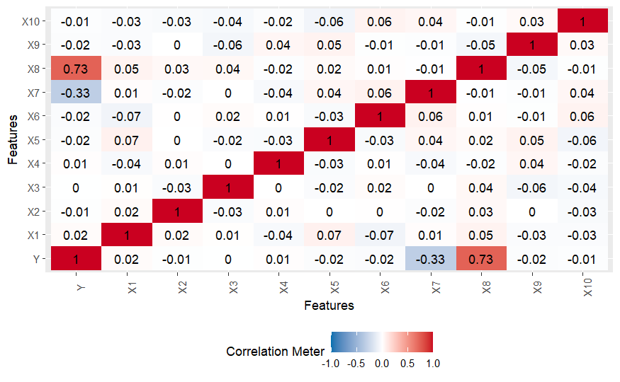
$X_7$ and $X_8$ have high correlation to $Y$. They seem to be an important predictor.
The QQ-Plot shows an S-shaped pattern. Maybe it violates the assumption of linear regression.
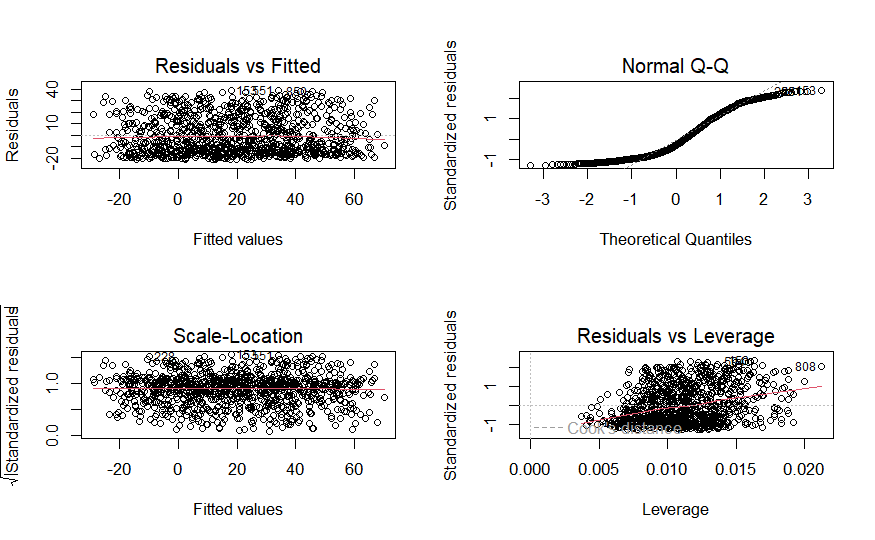
We use residual plot to diagnose. We find that the plot residual against $X_3$ shows a curved pattern.
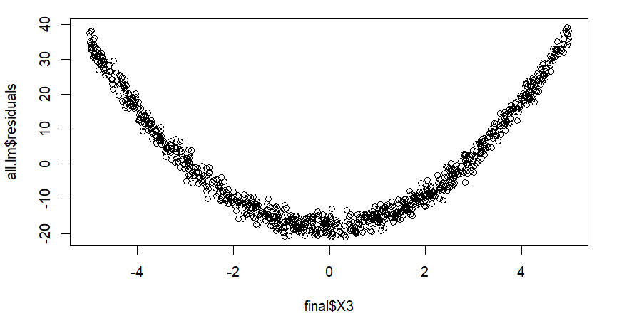
$$Y = X_1 + X_2 + X_3 + X_4+ X_5 + X_6 + X_7 + X_8 + X_9 + X_{10} + X_3^2$$There are 11 variables, and $2^{11}$ possible model. Accordingly, we use backward stepwise. What’s more, AIC in each step is decreasing.
The final model is $Y = X_1 + X_7 + X_8 + X_9 + X_{10} + X_3^2$ with R-squared $0.9986$ . Hence, it is the appropriate model.
The value of $X_8,\ X_9,\ X_{10}$ are unknown, so we assume it is zero. We want to estimate $Y$ by the new data. Using the prediction interval, we have $90 \%$ confidence that
$Y \in [5338.02,\ 5373.58]$